After preprocessing, the next step is to identify the Most Variable Genes (MVG). Single-cell datasets often contain thousands of cells and tens of thousands of detected genes. However, many of these genes are not informative for downstream analysis. MVG selection reduces the dataset to the most biologically relevant genes, improving the quality of clustering and embedding.
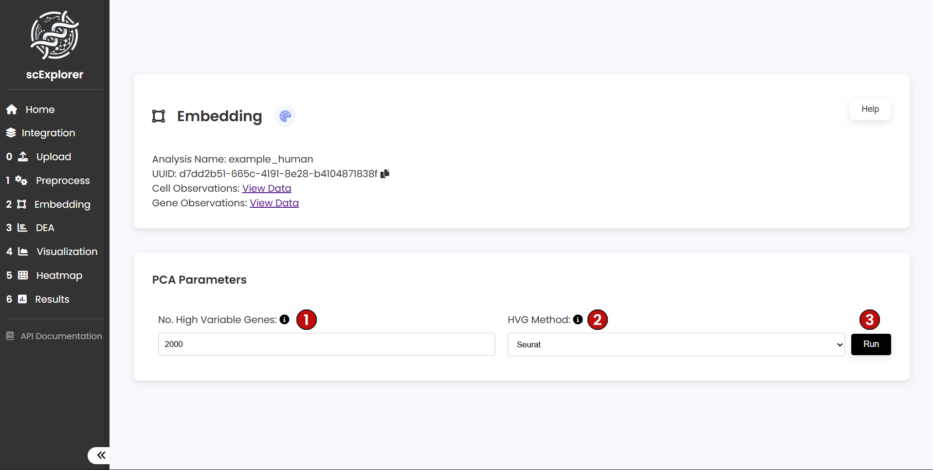
In (1), specify the number of genes you want to keep. Then choose the method for MVG calculation (2). scExplorer offers two methods: Seurat and Cell Ranger. For this tutorial, we will select 2000 MVG using the Seurat method (default parameters). Once set, click Run (3) to continue.
The number of optimal MVG will depend on the complexity of the dataset. Usually, a range between 1,000 and 5,000 MVG works well across single-cell data. Thus, we encourage users to test different numbers of MVG.
MVG should be determined after quality control, to guarantee that low-expressed genes and low-quality cells do not interfere with the analysis. Also, it is important to determine whether the data has technical noise to avoid selecting MVG for only one batch. If your data has batch effect, you can correct and integrate it in the Integration section.
We offer two methods for MVG selection: Seurat and Cell Ranger.
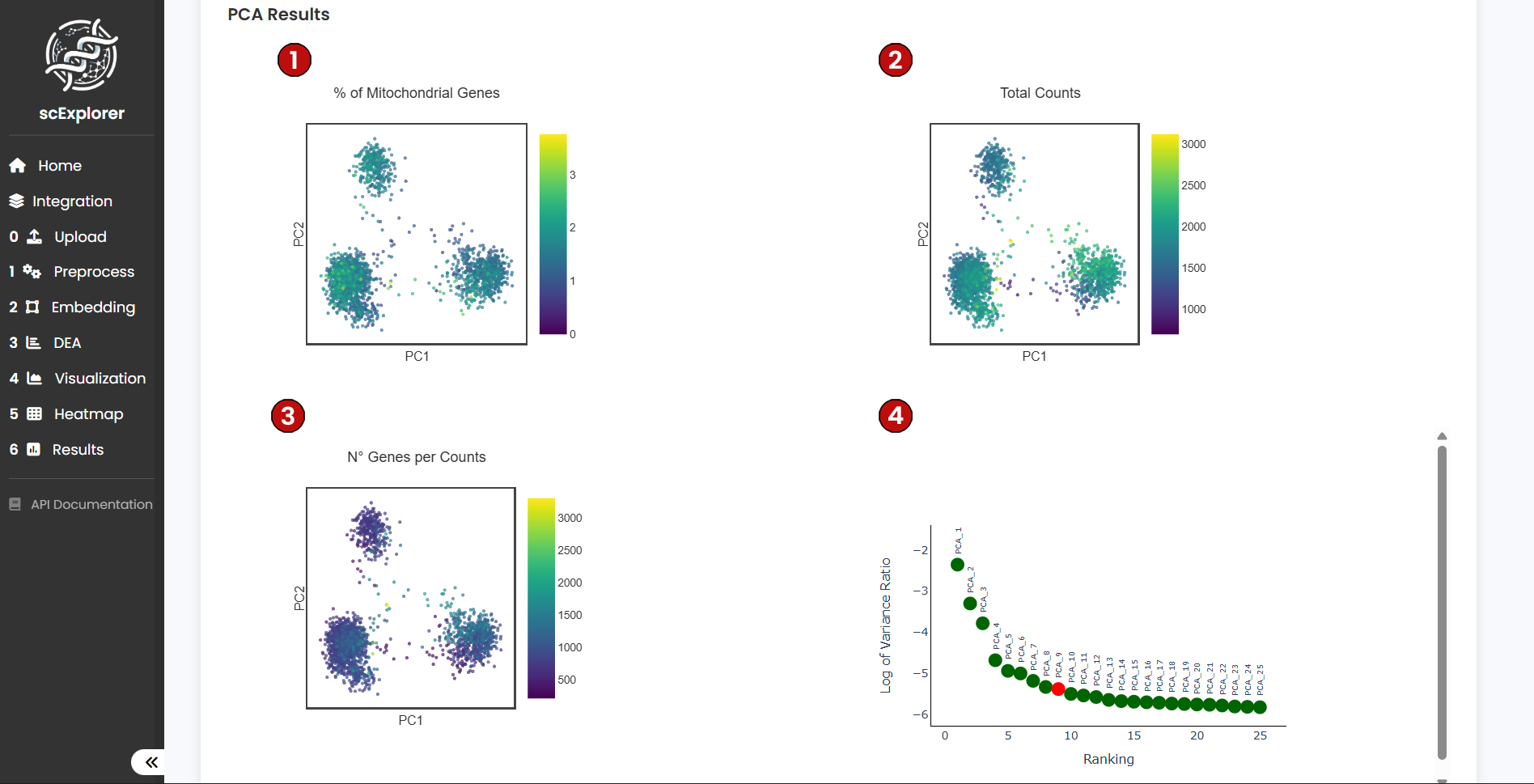
After running the analysis, you will see three plots for PC1 and PC2 highlighting:
Plotting the top 2 PCs is useful to see undesired features such as batch and QC metrics generating significant variation in your dataset. In (4) you can see the top 25 PC ranked according to the Variance Ratio and in red the suggested number of PC to be used for downstream analysis. For this tutorial, we will use the first 10 PC but we encourage users to explore using more or less PC.
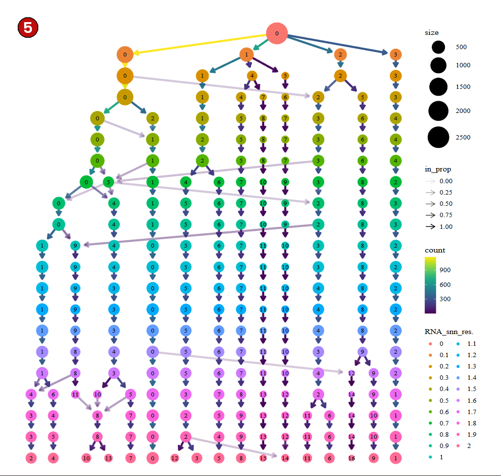
In addition, below you will find a clustree (5) which is a commonly used tool (particularly in R/Seurat) to explore and interpret how clusters change across different levels of clustering resolution. This visualization is especially useful when you apply clustering algorithms, like Louvain or Leiden, which allow for tuning a resolution parameter that influences the granularity of the resulting clusters. Here, clustree is calculated using a Shared Near Neighbors (SNN) graph and will be useful for users to use it as a reference during the construction of the K-Near Neighbors (KNN) graph downstream.
In the context of single-cell genomics, a principal component (PC) is a mathematical construct derived from principal component analysis (PCA), a dimensionality reduction technique used to simplify complex datasets.
Each PC represents a direction in the data that captures as much variance as possible. The first principal component (PC1) captures the most variance, the second principal component (PC2) captures the second most, and so on, with each subsequent component being orthogonal (uncorrelated) to the others.
PCA is useful in single-cell genomics because of the high-dimensional nature of the data, where each cell is represented by thousands of gene expression values. By reducing the data to just a few principal components, you can visualize the relationships between cells in a lower-dimensional space without losing much of the information.
Once you are satisfied with the PC analysis, the next step is to construct the KNN graph from the desired number of PCs and embed in two dimensions for visualization with Uniform Manifold Approximation and Projection (UMAP).
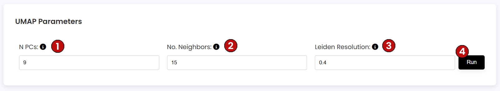
Parameter settings:
For this tutorial, we will set the number of PC to 9, number of neighbors to 15, and Leiden resolution to 0.4 . We encourage users to explore multiple parameters. Click on Run (4) to generate the UMAPs.
In single-cell genomics, both the Louvain and Leiden algorithms are widely used for clustering cells based on their gene expression profiles. These algorithms help identify groups of cells (clusters) that share similar gene expression patterns, representing distinct cell types or states within a complex dataset.
Why Leiden is preferred over Louvain:
The number of neighbors (K in KNN): This critical parameter influences how cells are grouped and visualized. Low K creates tighter, more localized neighborhoods (fine-grained clusters), while higher K values create more connected graphs (broader clusters).
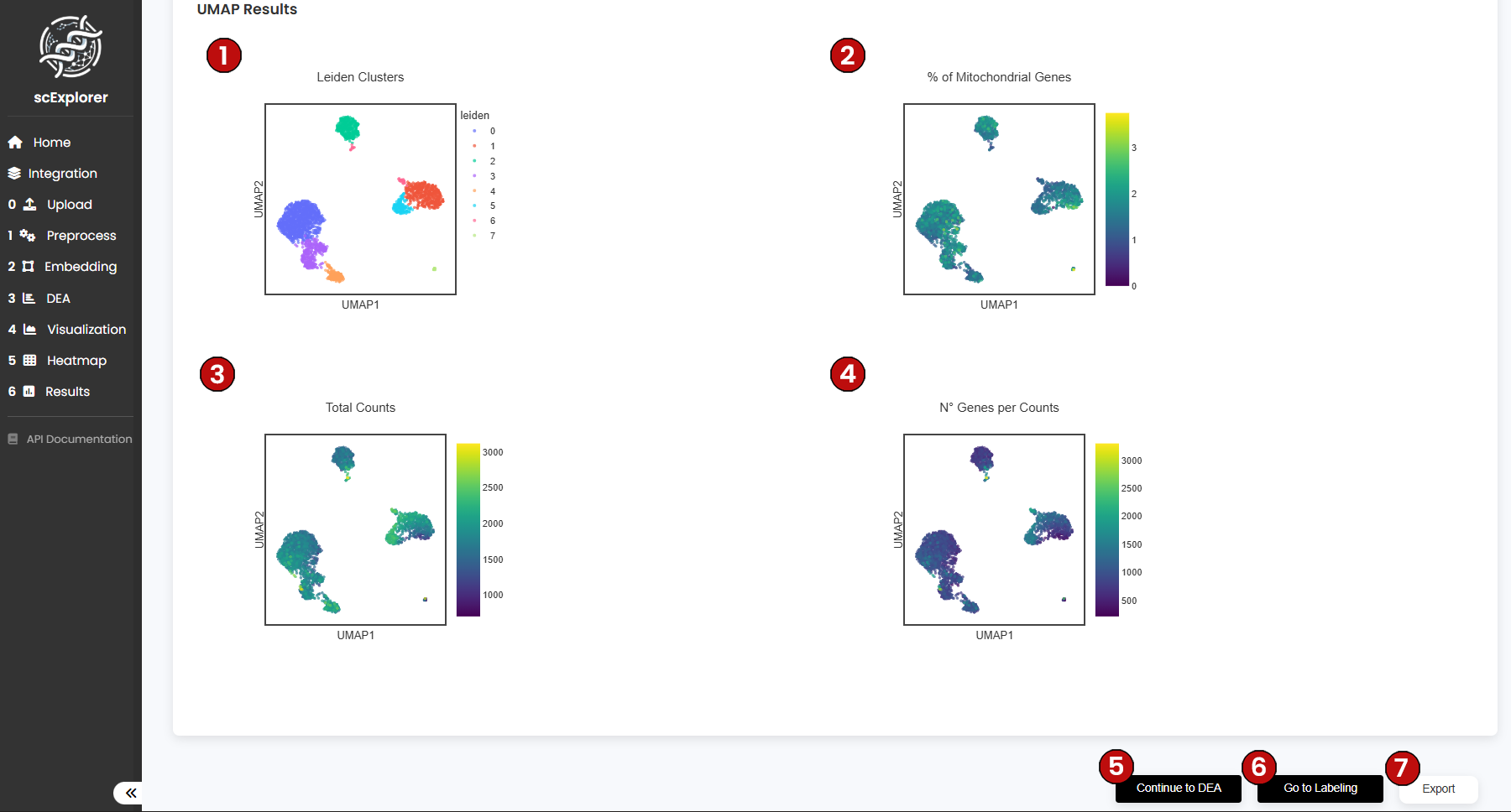
UMAP Is a dimensionality reduction technique widely used in single-cell genomics to visualize high-dimensional data in a lower-dimensional space. UMAP is particularly adept at preserving both the global and local structure of the data, making it a powerful tool for uncovering patterns and relationships in the high-dimensional space.
After running the analysis, scExplorer will show four UMAPs:
Next, click on DEA (5) to continue to the Differential Expression Analysis (DEA).